Introduction

Many gamers, when tweaking their graphics settings, come across options like Texture Filtering, Bilinear Filtering, and Anisotropic Filtering. Most people crank them up to maximum without really knowing what they do — or why turning them down makes distant floors shimmer and fences show strange flickering patterns.

If you dig deeper, you’ll find that these settings sit on top of a complete mathematical framework — the same one behind the Fourier transforms and convolution you might have seen in a signals and systems course.

This article traces that connection from start to finish. Starting from “what does texture filtering actually do,” we’ll work through:

• Why jaggies, flickering, and Moiré patterns appear
• Why MipMap is necessary
• Why sharp edges represent high frequencies
• What the Fourier Transform actually does
• Why convolution matters so much
• How all of these connect into one coherent picture

---

Part 1: What is Texture Filtering?

1.1 What Actually Happens During Texture Mapping

In graphics, we often paste an image onto the surface of a 3D model — that image is called a texture.

Examples:

• Brick patterns on a floor
• Stone texture on a wall
• Patterns on a character’s clothes
• Wear marks on a gun surface

When a triangle is textured, every fragment on screen gets a texture coordinate — a UV coordinate. The problem is:

• The screen is a discrete pixel grid
• The texture is a discrete texel grid
• But UV coordinates usually land at non-integer positions in the texture
• A single screen pixel doesn’t necessarily map to just one texel

This leads to a core question:

When a fragment needs to sample a color from the texture, how exactly should it do that?

That’s what Texture Filtering is about.

1.2 Understanding the Word “Filtering”

In everyday language, “filtering” sounds like “removing impurities.” But in graphics and signal processing, it’s closer to the concept of filtering / filtering operation:

Selecting, weighting, smoothing, or suppressing neighboring samples according to some rule, to produce an output that’s more appropriate for the current use case.

So in texture sampling, filtering isn’t about “retouching the image” — it’s about:

How should the current screen pixel combine nearby texture information to produce a reasonable color?

---

Part 2: Basic Texture Filtering Methods

2.1 Nearest Neighbor Filtering

The simplest approach: find the nearest texel to where the UV lands, and use its color directly.

Pros:

• Fast and cheap
• Pixel art games intentionally use this for the hard-edge look

Cons:

• Blocky appearance when magnified
• Flickering when minified
• Textures look “dirty” and jumpy

Its essence: represent the current location with just one sample, no smoothing.

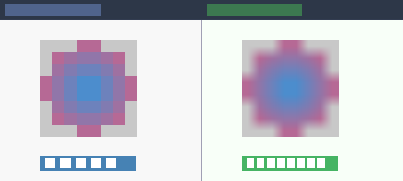
2.2 Bilinear Filtering

The more common approach. When the UV lands between 4 neighboring texels, instead of picking just one, it blends all 4 by distance-weighted interpolation.

• Interpolate along x first, then along y — hence “bilinear”

What it solves:

• Less blocky when magnified
• Smoother texture edges

What it doesn’t solve:

• Still flickers significantly when minified
• Dense textures still shimmer at a distance
• High-frequency detail still causes problems

Bilinear filtering is better, but it doesn’t truly fix the problem of many texels mapping to a single screen pixel when the texture is minified.

---

Part 3: Why Texture Minification Causes Problems

3.1 One Pixel Doesn’t Always Map to One Texel

Many beginners intuitively assume a screen pixel just samples one point on the texture. In reality, this is often not the case.

When an object is far from the camera:

• One screen pixel may correspond to a large area in texture space
• That area may contain many texels

Think of: distant brick floors, chain-link fences, window grilles, text decals. Up close they’re full of detail, but far away the screen can’t spare enough pixels for them.

3.2 What Happens Then

If you still just grab one sample from that large area (like Nearest Neighbor does), you get:

• Flickering
• Moiré patterns
• Shimmering / Crawling
• Jittering at a distance

Because:

You should be computing one representative value across a large texture region, but you’re only poking a single point somewhere in it.

---

Part 4: What is Sampling?

4.1 The Continuous World and Discrete Representation

Sampling means: from a continuous signal, you don’t look at every position — you pick samples at intervals.

Sampling is everywhere in graphics:

• Screen pixels are sampling a continuous scene
• Textures are sampling continuous surface colors
• Shadow maps are sampling light visibility
• Frame-by-frame rendering is temporal sampling

Graphics is fundamentally a sampling-driven discipline.

4.2 Why Sampling Causes Problems

Once you only look at discrete samples, you might miss things. If the signal changes slowly, sparse samples are fine. But if the signal changes quickly, sparse samples will definitely cause problems.

This “how fast it changes” is what we call frequency.

---

Part 5: The Sampling Theorem and Nyquist

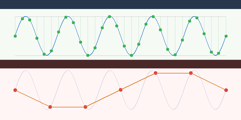
5.1 What the Sampling Theorem Says

The Nyquist-Shannon Sampling Theorem states:

If a signal’s highest frequency does not exceed f_max, then a sampling rate f_s of at least 2f_max is needed to unambiguously reconstruct the original signal from its samples.

Formula: f_s >= 2 * f_max

Where:

• f_s: sampling frequency
• f_max: maximum signal frequency

5.2 Plain Language Version

A memorable way to put it:

If something changes at a certain rate, you need to observe it at least twice as fast, otherwise you’ll see it wrong.

“Seeing it wrong” doesn’t just mean “missing some detail” — it means high-frequency information disguises itself as incorrect low-frequency information. This is called Aliasing.

---

Part 6: What is Aliasing?

6.1 Aliasing Isn’t “Lost Detail” — It’s “Wrong Detail”

Many people assume undersampling just loses information. The worse reality:

High-frequency signals fold into incorrect low-frequency patterns.

Meaning:

• You’re not seeing the original detail
• Nor just a blurry version
• But fake patterns, fake rhythm, fake oscillations

6.2 Aliasing in Graphics

The most common aliasing symptoms:

• Jagged edges (Jaggies) on polygon boundaries
• Flickering distant textures
• Moiré patterns
• Jumping shadow edges
• Distant fine grids or fences looking dirty

They look different on the surface, but share the same root cause: the signal frequency is too high for the sampling rate.

---

Part 7: Why Sharp Edges Represent High Frequency

7.1 What “Frequency” Means in Images

In images, spatial frequency refers to: how quickly the image content changes across space.

Examples:

• Large smooth gradients: low frequency
• Gradual brightness changes: low frequency
• Fine lines, fine textures: high frequency
• Sharp edges: high frequency — lots of it

7.2 Why Sharp Edges Are High Frequency

Imagine an image that’s fully black on the left, fully white on the right, with a very sharp boundary in between. That means brightness jumps from 0 to 1 over a very short spatial distance.

This “extremely fast change” requires high-frequency components to represent. Think of it this way:

• Low frequencies can only draw slow, smooth changes
• Abrupt, steep, sudden transitions require higher frequencies

Therefore: the sharper the edge, the more high-frequency content it contains. That’s why edges are the first to alias, and the first to suffer from sampling problems.

---

Part 8: Why MipMap Reduces Aliasing

8.1 What MipMap Is

MipMap is a series of precomputed versions of the same texture at decreasing resolutions:

1024 × 1024
512 × 512
256 × 256
128 × 128
...
1 × 1

Each level is half the size of the previous.

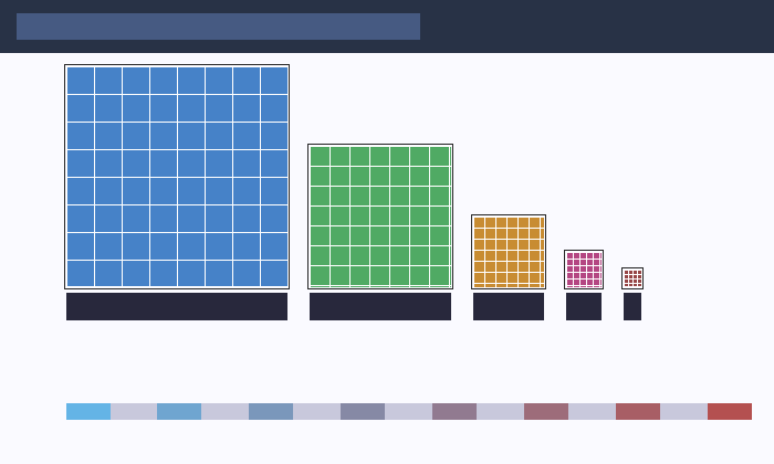
8.2 The Real Point of MipMap

On the surface, it looks like just a bunch of smaller copies. But at its core:

Before sampling at low resolution, it pre-averages the high-frequency detail away.

When an object is far away → the screen pixel can’t hold all the high-frequency detail from the full-res texture → don’t sample the high-res texture blindly → use a pre-“low-passed” lower-resolution version instead.

8.3 MipMap and the Sampling Theorem

This is exactly the standard procedure the sampling theorem requires: before downsampling, you must apply a low-pass filter.

Why? Because if you don’t remove frequencies that exceed what the sampling rate can handle, aliasing is inevitable.

MipMap pre-computes the “low-pass then downsample” process and stores it as multiple levels for fast runtime lookup.

One-sentence summary: MipMap is the engineering implementation of the sampling theorem for texture systems.

---

Part 9: Trilinear and Anisotropic Filtering

9.1 Trilinear Filtering

Bilinear filtering only interpolates within a single Mip level. But the ideal resolution often falls between two adjacent levels.

Trilinear filtering:

1. Does bilinear sampling on two adjacent Mip levels
2. Then interpolates between those two results

It solves: hard transitions between Mip level switches.

9.2 Anisotropic Filtering

MipMap makes a simplifying assumption: a screen pixel’s footprint in texture space is roughly square.

But when viewing a surface at an oblique angle, the footprint is stretched — one direction needs higher resolution, another direction needs more averaging.

Anisotropic filtering takes multiple samples along the major axis of the footprint, more accurately approximating the true texture coverage.

Quick summary:

• Trilinear: smooth transitions between Mip levels
• Anisotropic: handle pixels whose texture footprint is stretched, not square

---

Part 10: How This All Leads to “High/Low Frequency”

Chasing the root cause of texture filtering, MipMap, and anisotropic filtering always leads back to the same question:

What detail frequencies can the current sampling rate handle?

This makes “what frequency components does this image contain” a critical question. And that naturally leads us to Fourier Analysis.

---

Part 11: What is the Fourier Transform?

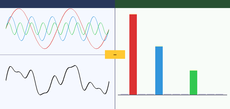
11.1 One-Sentence Definition

The Fourier Transform’s essence:

Rewriting a signal described by position or time into a description of “what frequencies it’s made of.”

• Before: you see the value at each position
• After: you see which frequencies exist, and how strong each one is

This is fundamentally a change of coordinate system.

11.2 Why Go to the Frequency Domain?

Because many things that are hard to see in the original space become immediately clear in the frequency domain:

• Why blurring makes images soft
• Why sharpening enhances edges
• Why edges represent high frequencies
• Why undersampling causes aliasing
• Why MipMap needs low-pass filtering

11.3 What Are Low and High Frequencies?

Think of an image as the superposition of many waves at different speeds:

• Low-frequency waves: change slowly, carry overall shapes and large-scale brightness
• High-frequency waves: change quickly, carry fine details, edges, and textures

So:

• Smooth regions: dominated by low frequencies
• Detail regions: more high frequencies
• Sharp edges: packed with high frequencies

---

Part 12: Why Sine Waves Are a Natural Basis for Analysis

12.1 Why Sine Waves?

Fourier analysis uses sine and cosine waves as its basis because:

1. They’re mathematically simple
2. Different frequencies are mutually orthogonal
3. Many systems have simple responses to sine waves
4. Complex signals can be seen as sums of these waves

12.2 What Does “Orthogonal” Mean Here?

It doesn’t mean “perpendicular on a graph” — it means:

Under a well-defined inner product, the two functions don’t mix with each other.

For functions, the inner product is typically: <f, g> = ∫ f(x) g(x) dx

If it equals zero, the functions are orthogonal. In the Fourier series, sine/cosine functions of different frequencies are mutually orthogonal — meaning one frequency component doesn’t contaminate another, allowing clean decomposition.

12.3 Orthogonal vs. Linearly Independent

• Linearly independent: no element is a linear combination of the others (no redundancy)
• Orthogonal: linearly independent, and also mutually perpendicular under the inner product

Orthogonality is strictly stronger. Fourier analysis is so useful largely because its basis is not just linearly independent, but orthogonal.

---

Part 13: What Does the Frequency Domain Give Us?

The Fourier transform result tells us: which frequencies exist, how strong each one is, how the image’s frequency components are distributed.

This lets us understand phenomena through a frequency lens:

• Blurring: suppresses high frequencies
• Sharpening: boosts high frequencies
• Undersampling: folds high frequencies into incorrect low frequencies
• Edges: lots of high frequency
• MipMap: removes excess high frequencies before low-rate sampling

Many “image quality” problems in graphics are fundamentally frequency problems.

---

Part 14: What is Convolution?

14.1 One-Sentence Definition

Slide a small template (kernel) over the signal or image; at each position, compute the weighted sum of nearby neighbors to produce the output for that position.

Think of convolution as: structured mixing of the local neighborhood, where the mixing rule is defined by a convolution kernel.

14.2 Why Convolution?

We often want to do things to images:

• Blur
• Sharpen
• Edge Detection
• Denoise
• Feature Extraction

These all share a common trait: the output at a position depends not just on that position, but on its neighborhood. That’s exactly what convolution naturally expresses.

---

Part 15: What is a Convolution Kernel?

A kernel is just a set of weights that determines:

• Which neighbors matter more
• Whether to average or differentiate
• Whether to smooth, sharpen, or detect edges

Mean blur kernel (3×3):

1/9 * [[1,1,1],
        [1,1,1],
        [1,1,1]]

Looks at 9 surrounding pixels, averages them — the image becomes smoother.

Gaussian kernel: Center weight is largest, decreasing with distance. More natural than simple averaging.

Edge detection kernel: One side positive, one side negative — emphasizes change. The 1D difference kernel [-1, 1] highlights positions where values change rapidly, i.e., edges.

---

Part 16: Why Convolution and Filtering Are So Closely Tied

Because many filtering operations can essentially be written as convolution:

• Blur = Low-pass filtering
• Sharpening = Emphasizing high frequencies
• Edge detection = Extracting high-frequency changes
• Image smoothing = Weighted neighborhood average

Convolution is the standard mathematical form for implementing local filtering operations.

---

Part 17: Why Convolution and Fourier Transform Are So Deeply Related

There’s a critical result called the Convolution Theorem:

Convolution in the spatial/time domain corresponds to multiplication in the frequency domain.

Meaning:

• Sliding a kernel over the image in spatial space
• Is equivalent to multiplying each frequency by a weight in the frequency domain

17.1 Why Blurring Suppresses High Frequencies

A blur kernel in the frequency domain typically multiplies low frequencies by values near 1, and high frequencies by smaller values. Result: large-scale shapes are preserved, fine details and edges are weakened.

Blurring is fundamentally low-pass filtering, and low-pass filtering can be implemented via convolution.

17.2 Why Sharpening Enhances Edges

Sharpening kernels typically keep the center, apply negative weights to neighbors — emphasizing how much the current position differs from its surroundings. In frequency terms, this boosts high-frequency content, and high frequencies are where edges and details live.

---

Part 18: Putting the Whole Chain Together

We can now trace the complete path from texture filtering to convolution:

1. Texture filtering asks: how should a screen pixel sample the texture?
2. Minification problems reveal: one pixel may map to many texels
3. This is fundamentally a sampling problem
4. The sampling theorem tells us: insufficient sampling rate causes aliasing
5. So we must first apply low-pass filtering
6. MipMap is the engineering solution for pre-filtering textures
7. To understand low-pass, high/low frequency, and edges, we need Fourier Transform
8. Fourier tells us: edges and details = high frequency
9. To actually implement these local filtering operations on images, we need convolution
10. The convolution theorem connects spatial and frequency domains

The vast majority of image quality problems in graphics share a root cause: how to correctly represent a continuous signal containing high-frequency detail using a finite sampling rate. Texture filtering, MipMap, Fourier Transform, and convolution form one complete toolkit for addressing this.

---

Part 19: One-Liner Reference

Concept	One-liner
Texture filtering	How a screen pixel samples a color from the texture
Bilinear filtering	Interpolate from 4 nearby texels
MipMap	Don’t sample the full-res texture at distance — use a pre-filtered version
Anisotropic filtering	Fix the problem that a pixel’s texture footprint isn’t always square
High frequency	Rapidly changing detail, edges, fine textures
Low frequency	Slowly changing large shapes, smooth regions
Sampling theorem	Sampling rate must be at least twice the signal’s highest frequency
Aliasing	High frequencies disguised as incorrect low frequencies
Fourier Transform	Rewrite a signal from position/time description to frequency description
Convolution	Slide a local weight template over the image, computing weighted sums
Convolution theorem	Spatial-domain convolution = frequency-domain multiplication

---

Part 20: Closing Thoughts

Many beginners see these concepts as belonging to different fields. But once you truly understand them, you’ll realize they’re not isolated knowledge points — they’re a shared language built around sampling and frequency.

Natural next steps if you continue deeper:

1. How does the GPU automatically select Mip level using ddx/ddy?
2. Why is Gaussian blur separable?
3. Why does TAA (Temporal Anti-Aliasing) fundamentally relate to sampling?
4. Why do shadow maps, normal maps, and SSR (Screen Space Reflections) all face similar frequency problems?

At that point, you’ll realize that the truly hard parts of graphics are often not “how to call the API” but:

Whether you genuinely understand sampling, frequency, and reconstruction.

• Graphics
• Signal Processing
• Fourier Transform
• Convolution
• MipMap
• Texture Filtering